I have a worksheet where column A has various names in varying formats:
A1 John Smith
A2 Jones, Mary
A3 Sally Gomez
A4 The Gonzalez family
Column B has similar data:
B1 The Smith Family Trust
B2 Bob and Mary Jones
B3 Blackwell, John
B4 Luz Gonzalez
I would like to identify the instances where the same last name is found in column A and column B. In the examples above, the formula, if placed in column C, would result in
C1 TRUE (because "Smith" is found in both A1 and B1)
C2 TRUE (because "Jones" is found in both A2 and B2)
C3 FALSE (because there are no common words between A3 and B3)
C4 TRUE (because "Gonzalez" is found in both A4 and B4)
Is this even possible?
Asked
Active
Viewed 4,164 times
3
candez
- 31
- 1
- 3
4 Answers
2
Given your comments as well as your question, it seems you want to return TRUE if any word in one phrase matches a word in the adjacent phrase. One way to do this is with a User Defined Function (VBA). The following excludes any words that are in arrExclude, which you can add to as you see fit. It will also exclude any characters that are not letters, digits or spaces, and any words that consist of just a single character.
See if this works for you.
Another option would be take a look at the free fuzzy lookup add-in provided by MS for excel versions 2007 and later.
To enter this User Defined Function (UDF), alt-F11 opens the Visual Basic Editor.
Ensure your project is highlighted in the Project Explorer window.
Then, from the top menu, select Insert/Module and
paste the code below into the window that opens.
To use this User Defined Function (UDF), enter a formula like
=WordMatch(A1,B1)
in some cell.
EDIT2: Find Matches segment changed to see if it works better on Mac
Option Explicit
Option Base 0
Option Compare Text
Function WordMatch(S1 As String, S2 As String) As Boolean
    Dim arrExclude() As Variant
    Dim V1 As Variant, V2 As Variant
    Dim I As Long, J As Long, S As String
    Dim RE As Object
    Dim sF As String, sS As String

'Will also exclude single letter words
arrExclude = Array("The", "And", "Trust", "Family", "II", "III", "Jr", "Sr", "Mr", "Mrs", "Ms")

'Remove all except letters, digits, and spaces
'remove extra spaces
'Consider whether to retain hyphens

Set RE = CreateObject("vbscript.regexp")
With RE
    .Pattern = "[^A-Z0-9 ]+|\b\S\b|\b(?:" & Join(arrExclude, "|") & ")\b"
    .Global = True
    .ignorecase = True
End With

With WorksheetFunction
    V1 = Split(.Trim(RE.Replace(S1, "")))
    V2 = Split(.Trim(RE.Replace(S2, "")))
End With

'Find Matches
If UBound(V1) <= UBound(V2) Then
    sS = " " & Join(V2) & " "
    For I = 0 To UBound(V1)
        sF = " " & V1(I) & " "
        If InStr(sS, sF) > 0 Then
            WordMatch = True
            Exit Function
        End If
    Next I
Else
    sS = " " & Join(V1) & " "
    For I = 0 To UBound(V2)
        sF = " " & V2(I) & " "
        If InStr(sS, sF) > 0 Then
            WordMatch = True
            Exit Function
        End If
    Next I
End If

WordMatch = False

End Function
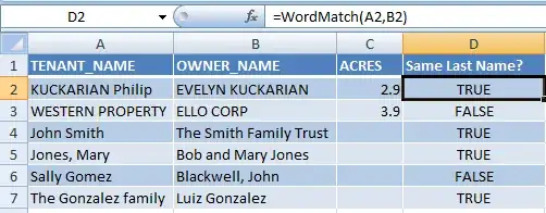
EDIT: Here is a screenshot of the results, using both your original examples, and also the examples you gave in a comment below where you indicated you were having a problem.
Ron Rosenfeld
- 8,198
- 3
- 13
- 17
-
This seems like it should work but I'm getting a #VALUE! error. – candez May 07 '15 at 07:40
-
Please provide (copy/paste the two strings) an example where a `#VALUE!` error is being returned by UDF. – Ron Rosenfeld May 07 '15 at 10:49
-
TENANT_NAME OWNER_NAME ACRES Same Last Name? KUCKARIAN, PHILLIP EVELYN KUCKARIAN 2.9 #VALUE! WESTERN PROPERTY ELLO CORP 3.9 #VALUE! Is this what you are looking for? In the first row, the UDF should have returned TRUE, and in the second row FALSE. I can also upload a screen shot if that would be more helpful. (and thank you for your help) – candez May 08 '15 at 07:50
-
@candez I have added a screen shot showing the UDF working with the examples you provided. Are you certain that both arguments of the UDF refer to cells that are not empty? Are you certain you placed the UDF in a Regular Module as per the instructions? – Ron Rosenfeld May 08 '15 at 10:30
-
Hmm. I am clearly doing something wrong. I'm using Excel for Mac 2011, if it makes a difference. This is how it appears when I enter the script [link](http://candacernelson.com/images/misc/Script.jpg), and this is where I have entered the UDF [link](http://candacernelson.com/images/misc/Code.jpg). When I hover over the #VALUE! error, it indicates "A value used in the formula is of the wrong data type." The text was in a General format, so I switched those columns to Text, but I'm still getting the error. – candez May 09 '15 at 03:15
-
@candez I am not sure why it works here and not on your machine. It is possible there is an issue in the `Find Matches` segment with `Application.Match` behaving differently in the two versions. I will edit my answer to provide a different method (using Regular Expressions) to check for matches, and see if that works better on your machine. – Ron Rosenfeld May 09 '15 at 11:07
-
@candez Edited again so as not to use Regex for the comparison. I think this version will be more bullet-proof. – Ron Rosenfeld May 11 '15 at 19:01
1
The most difficult part of this exercise is determining what, in column A, constitutes a last name. In your example, it's either:
- The first word, if there's a comma in the whole name
- The second word
If that rule is true, then you can just do a formula like this:
=NOT(ISERROR(FIND(last_name, B1:B4)))
The formula to actually determine the last name is a little more complex. You essentially have to figure out what character positions the spaces are in, and then pull the letters in between. There's a good explanation on this thread:
Will Ediger
- 143
- 8
-
Unfortunately there is no real pattern to what the last name is, as there are examples like "Bob and Mary Smith" or "Bob L Smith Et Al" or "Smith Bob L and Mary" with no comma. But this gives me a direction to head in. Thank you. – candez May 02 '15 at 09:04
-
1Actually in most cases, a TRUE value any time any single word is repeated, could work. It wouldn't be perfect, as it would incorrectly return a TRUE value when comparing "Bob and Mary Smith" and "John and Linda Jones," or "Bob L Smith" and "Jones, Bob" as TRUE. But in the majority of cases it could work. – candez May 02 '15 at 09:14
0
-
That isn't applicable to this problem. The solution you referenced is for an exact match of the entire cell contents. The problem here is for a match of any word that is a portion of the cell. – fixer1234 May 03 '15 at 20:07
0
Highlight both columns > conditional formatting (home tab) > highlight cell rules > duplicate values.
This will highlight all duplicates in both columns.
Make sure you are highlighting the columns and not the cells.
bummi
- 1,703
- 4
- 16
- 28
Doug Fresh
- 1
- 1
-
Doesn't this compare the entire cell contents rather than finding a matching word that is a portion of each cell? – fixer1234 May 03 '15 at 20:10
-
The other challenge with this is that I can't use the results in a formula. Ultimately I would like to create a SUMIF formula based on the TRUE or FALSE result in column C. – candez May 07 '15 at 05:36