How can I group row values sum them and turn them into column?

Question

I have a table where I have various costs that have been grouped can captured by row.

In the rows structure in the first row is the value I want to remain as a row, the second column has the transformed column name and the third row the value to sum.

This is a little like this question Excel: How to extract group of the same rows and their values into columns? but I want to include sums and power query would provide a suitable answer.

Prior to transform

Location	Expense Type	Description	Value
City 1	Food	Burger	100
City 1	Food	Sausages	50
City 1	Transport	Hover bike	1000
City 2	Entertainment	Cinema	320
City 2	Food	Brocoli	15
City 2	Transport	Bus	22
City 2	Transport	Train	8

After Transform

Location	Food	Transport	Entertainment
City 1	150	1000	0
City 2	15	30	320

Looking for the optimum way to do this, ideally it would handle additional entries without having to adjust the formula this will drive a subsequent vlookup.

What problem did you run into when you tried the Table.Pivot method in Power query (or even a simple Pivot Table in Excel)? Either would provide the results you show in your question. — Ron Rosenfeld, May 08 '23 at 02:07
When I tried to use the pivot function it ended up with a whole heap of nulls, I'm probably missing some small detail, hence im looking for an example — user1605665, May 08 '23 at 04:59
According to your sample, the general pivot table is helpful. **Locations** is Row field, **Expense Type** is Column field and **Value** is Values field. — Emily, May 08 '23 at 08:35
If you used Power Query, please edit your post to show the code you used (copy/paste from the Advanced Editor), so we can tell what you are doing incorrectly. It seems pretty straightforward from your data. — Ron Rosenfeld, May 08 '23 at 10:16
@Emily I don't want to use a pivot table, the out put needs to be an independent table. And not copy pasting aftewards — user1605665, May 09 '23 at 00:36
@RonRosenfeld i worked out the problem, in the real example there were a number of extra columns. They were messing with the pivot so I removed those columns from the query and it worked. I'll update the question and then answer it for future ref — user1605665, May 09 '23 at 05:00

score 0 · Answer 1 · answered May 11 '23 at 10:54

Can be done using power query

Power Query Code

 let
    Source = Excel.CurrentWorkbook(){[Name="Table1"]}[Content],
    #"Changed Type" = Table.TransformColumnTypes(Source,{{"Location", type text}, {"Expense Type", type text}, {"Description", type text}, {"Value", Int64.Type}}),
    #"Removed Columns" = Table.RemoveColumns(#"Changed Type",{"Description"}),
    #"Pivoted Column" = Table.Pivot(#"Removed Columns", List.Distinct(#"Removed Columns"[#"Expense Type"]), "Expense Type", "Value", List.Sum)
in
    #"Pivoted Column"

Step by step instructions

Select the Range
Select "Data from the menu"
Select "From Table / Range"

Remove the description column

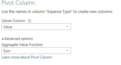
Select the column "Expense Type" then select pivot
On pivot chose "Value" as the value column and sum in the aggregation

The column would have pivoted, so now click close and load (under file)

How can I group row values sum them and turn them into column?

1 Answers1